Before we dive into arbitrage pricing, we can explore the more intuitive pricing methodology called “Expectation Pricing”. Its quite intuitive and often confused with arbitrage pricing.
Suppose you are playing a game of dice. The rule of the game is really simple. You pay a charge to play the game. You roll the dice. Suppose you roll a 4, 4$ will be returned. What should be the charge to play this game?
Mathematically, its supposed to be 3.5$ for each play. This number comes from the expectation of 1 through six with equal probability of .
But, we are forgetting one crucial part of the game. Its human psychology. People tend to spend less on things that can give them a loss. This behaviour is called risk aversion. People who play the game will not be willing to pay 3.5$. They will be willing to pay something less. How less? It depends on the person. Some are willing to pay only 2$ but a few might be willing to pay 3$.
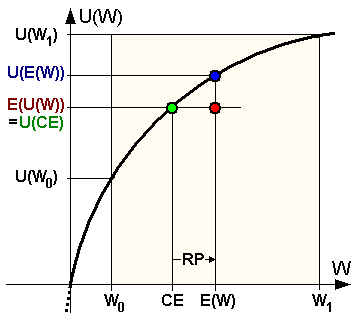
Given below is the Utility function of a risk averse investor. From the above example, $ but the is more than . CE is certainty equivalent. It is the equivalent amount that a risk averse is willing to spend to get the same utility as of a risk neutral investor. In the above scenario, it was 2$ for investor and 3$ for another). The gap between CE and E(W) is called the Risk Premium (RP).
In the above game, it was easier to calculate expectation because there are 6 faces for a die with equal probabilities. But, how do you calculate the expected value of a stock sometime in the future. There is literally infinite prices it can take and some price ranges are more probable than others. Do we need to make a probability curve to figure that out?
The answer is a big NO.
Suppose I want to buy a particular stock with current price of , sometime in the future, say, 1 year from now. What should be the price I would pay the seller one year from today?
Mathematically, let’s say I need to pay him K, one year from now:
Since I am getting into a forward contract with him, I will not be paying anything today. I will be paying K at the end of one year in exchange for the stock. Solving the above equation, I will get K as the following:
The mathematical genius in you is happy. You found the answer to be rather intuitive. Its saying you need to pay the seller “Expected Pricing” of the stock price at the end of one year. But, how do you go about calculating this?
You can create a probability curve, but there is no way you can verify anything that is in the future. So, although the methodology has no theoretical fallacy, its just not practical enough. There is no sure shot way of saying what K should be.
Here is where arbitrage comes to the rescue. One thing the mathematical way of looking at prices didn’t take into account is that we can buy the stock today and hold it till end of the contract. That way, we can agree that price is going to be the financing cost of buying and holding.
If someone quotes higher price than this, people are not going to be in contract with that seller because nobody wants to pay more. If someone quotes less than this, you can get into a contract with that seller, short the stock, put the fund in money-market and at the end of the contract, pay K`(< K) and pocket the difference (arbitrage).
So, the above price is the correct price. Because if the seller offers any other price, you can make a guaranteed profit from the trade.
It turns out, the way we constructed the price K from buy and hold strategy can be used to price almost every derivative. Particularly, options can be priced in a similar way.