Martingale Measures by examples

What is a measure?

A measure is a broad term. It means a consistent way of assigning weights to outcomes so that they add up correctly. The measure we are interested in is probability measure. So, for each possible event, there are a number of possible ways of assigning probability. All of those ways are a valid measure, if they add up to one and if there are no negative probabilities.

Imagine you write down every possible price path a stock could take over the next year — every wiggly trajectory from today to expiry. There are infinitely many of them. A measure is simply a rule that assigns a probability weight to each of these paths. It answers the question: how likely is each scenario?

The real-world measure P is the assignment of weights that reflects how paths actually occur in nature, informed by the stock’s true expected return, investor risk appetite, and everything else going on in the economy.

Here is a concrete analogy. Suppose two people are betting on a biased coin. Person A (the real world) says heads comes up 70% of the time. Person B (a fictional world) says heads comes up 50% of the time. The coin flip itself, the physical event, is the same. Only the probability weight assigned to each outcome differs. That difference between Person A’s weights and Person B’s weights is a change of measure.

Why do we need to change the measure?

In finance, the real-world measure P is the natural one. Under P, a stock with expected return μ = 12% and risk-free rate r = 5% has a risk premium of 7%. This premium is what compensates investors for bearing uncertainty. It is real and economically important.

But here is the problem. When you try to price a derivative say, a call option, under the real-world measure P, you need to discount the expected payoff at a risk-adjusted rate. That risk-adjusted rate depends on investor risk preferences, which are unobservable and contested. Every investor has different preferences. Pricing under P requires you to know something you can never cleanly measure.

The insight of Black, Scholes, and Merton was that you can sidestep this entirely. Instead of working under P with a complicated risk-adjusted discount rate, you switch to a different measure Q, the risk-neutral measure, under which every asset earns exactly the risk-free rate. Under Q, pricing becomes:

No risk preferences needed. Just discount at r.

The Q measure is a mathematical convenience, a re-weighting of paths chosen specifically to make this formula work. It does not describe how the world actually is. It is a tool that makes the calculation tractable. The price you get is exactly the same as you would get under P with the correct risk adjustment, it is just far easier to compute.

Note:

Changing the measure does not change the price. It changes how hard the calculation is. Under Q, pricing derivatives reduces to taking a simple expectation and discounting at r.

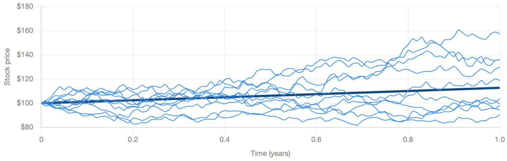
Geometric Brownian motion

Under the real-world measure P, we model the stock price using Geometric Brownian Motion (GBM). The stock evolves continuously in time according to:

The drift $μ·S·dt$ is the predictable part, the average direction the stock trends. The diffusion $σ·S·dW^P$ is the random part, the unpredictable noise driven by a standard Brownian motion $W^P$. This has an exact solution:

The term (μ − σ²/2) rather than μ appears because of Itô’s lemma, a correction that arises from the quadratic variation of Brownian motion. Intuitively, because the stock price is a nonlinear (exponential) function of the Brownian motion.

The following stock price simulation uses $S_0 = 100, \mu=12\%, \sigma=20\%$:

Changing the measure: Girsanov’s theorem

We want to move from the real-world measure P (where the stock drifts at μ) to the risk-neutral measure Q (where the stock drifts at r). The paths themselves do not change. We only change the probability weights assigned to each path.

The key quantity is the market price of risk θ — how much excess return the stock offers per unit of volatility:

Girsanov’s theorem says: define a new process

Under the re-weighted measure Q, $W^Q$ is a standard Brownian motion, zero drift, variance equal to time, all Brownian properties intact. The drift θ·t has been absorbed into the measure change, not into the paths.

Substituting back into the stock SDE: replace $dW^P = dW^Q − θ·dt$:

since μ − σθ = μ − (μ−r) = r,

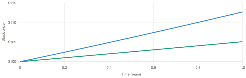
The drift changed from μ to r. The volatility σ is unchanged. The paths are the same wiggly trajectories, just re-weighted so that the upward-trending paths are now considered less likely, and the process appears to drift at exactly r.

The green line (mean under Q) hugs the risk-free growth line. Under Q, the stock is expected to grow at r, not because the world changed, but because we re-weighted the paths so the optimistic ones (high μ) became less probable and the pessimistic ones became more probable, exactly cancelling the risk premium.